Prepare Data For Machine Learning Using Amazon Sagemaker Data Wrangler
Demo Video
Coming soon!
Before You Begin
You must run the main Cloud Formation template and capture the following outputs from the Outputs tab.
-
Parameters for launching Sagemaker Studio cloud formation template.
- SageMakerRoleArn
- SubnetAPublicId
- VpcId
- TaskDataBucketName
-
Parameters for connecting to Redshift Cluster
- Cluster Identifier
- Database name
- Database User
- Redshift Cluster Role
Launch the following Sagemaker Studio cloud formation template by clicking the button below, and provide the parameter values listed in section 1 above (captured from the main template’s output).

Client Tool
This demo will use Amazon SageMaker Data Wrangler which can be accessed from Amazon SageMaker Studio.
Challenge
Kim (Data scientist) has been tasked to predict clients who are most likely to sign up for long term deposits. But the banking data set that Kim has received is not machine learning ready and Kim must analyze and cleanse the data before a Machine Learning Model can be trained.
Banking data set is related with direct marketing campaigns (phone calls). Campaigns are run to encourage clients to sign up for long term deposits. Banking data set contains client data, campaign data and socio-economic data. Before machine learning model is built Kim is going to analyze the data set and apply various data cleansing techniques like addressing missing values, encoding categorical variables and standardizing numeric variables.
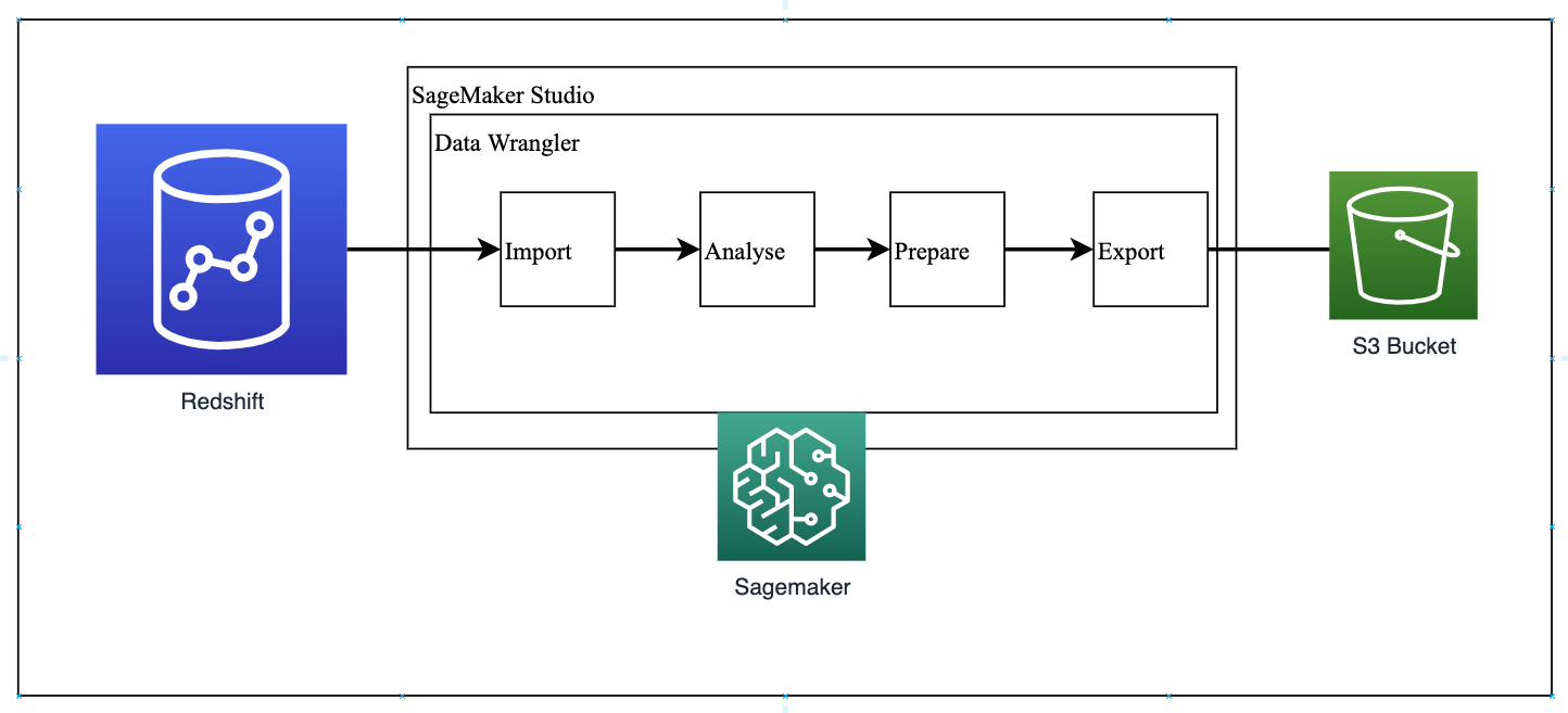
Banking data set is stored in Amazon Redshift Cluster. Kim plans to use Data Wrangler tool to connect to Redshift Data Warehouse and pull data to understand the data set and then work on data preparation process. Kim will have to do the following steps.
- Create new Data Flow
- Import Data set
- Analyze and Visualize
- Drop Unused columns
- Create Dummy Variables
- Standardizing Numeric Variables
- Export Processed Data
Data Wrangler Data Preparation - WorkFlow
Create new Data Flow
| Say | Do | Show |
|---|---|---|
|
We have banking data set stored on Amazon Redshift Data warehouse. Amazon Redshift makes it easy to gain new insights from all your data. Kim queries banking data set and does initial observation of the data set. From initial observations Kim identifies that Data set is not machine learning ready - for example, categorical variables like job and marital fields do not have reference variables which are required for Machine Learning. Kim decides to use |
Once the Studio stack is created, navigate to SageMaker Studio.
This will launch the Studio’s JupyterLab environment in a new browser tab (might take 2-3 minutes) |
|
|
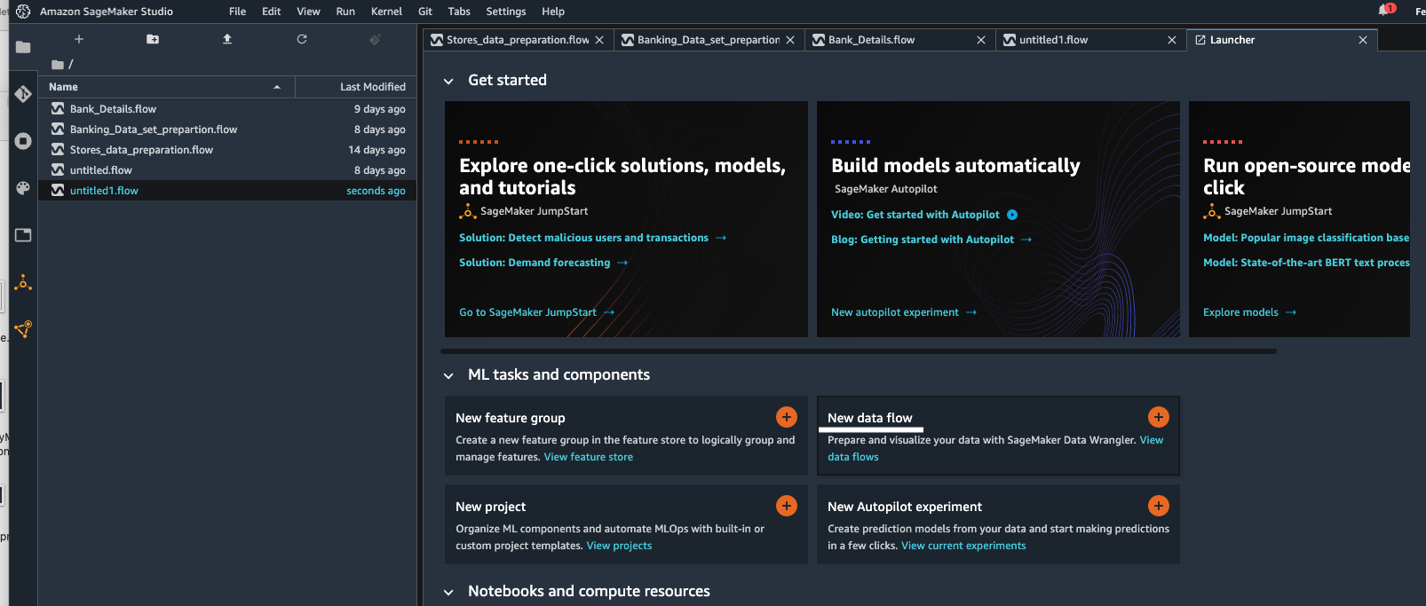
Amazon SageMaker Data Wrangler reduces the time it takes to aggregate and prepare data for machine learning (ML) from weeks to minutes. With SageMaker Data Wrangler, you can simplify the process of data preparation and feature engineering, and complete each step of the data preparation workflow, including data selection, cleansing, exploration, and visualization from a single visual interface. Kim starts by creating a new |
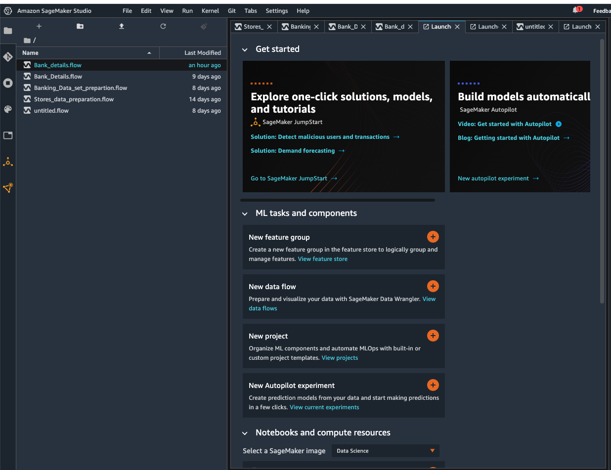
Goto Sagemaker studio.
This creates a new untitled.flow file. Kim decides to name this flow as Bank_details.flow. |
|
Import Data set
| Say | Do | Show |
|---|---|---|
|
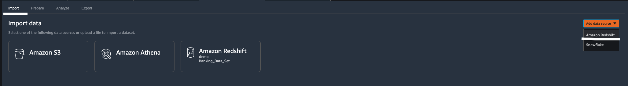
As a first step Kim makes a connection to her Cloud Data warehouse Amazon Redshift. Amazon Sagemaker Data Wrangler built in out of the box feature makes it real easy to connect to Amazon Redshift. |
Go to Import tab in Banking_Datails.flow
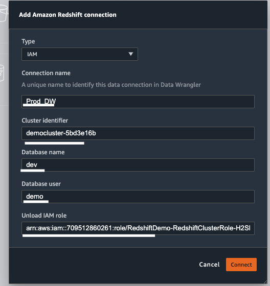
A new window Add Amazon Redshift Cluster opens up, choose following
|
|
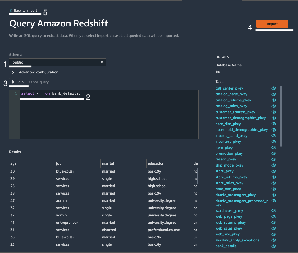
| After successful connection, Kim wants import her Bank_details data set into data wrangler. |
After successful connection to Redshift Cluster, “Query Amazon Redshift” page is displayed
Go to Schema and Select Public schema from drop down list.
|
|
|
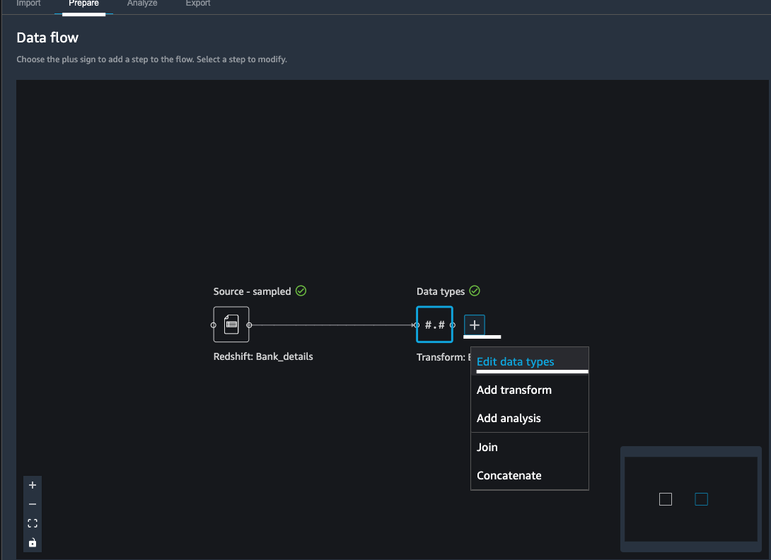
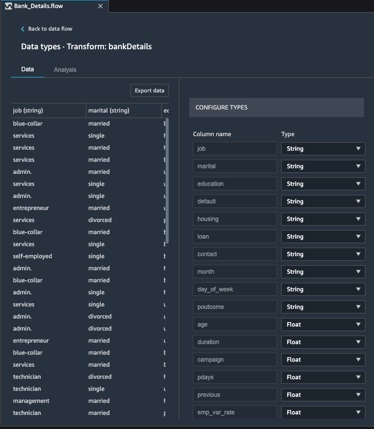
Kim now wants to know more details about her data set. For example, she wants to understand data types of the data set that she has imported. Data wrangler automatically infers the type of data for each column. Kim wants to make sure data types are correctly set for each column. |
Under Data flow tab
|
|
Analyze and Visualize
| Say | Do | Show |
|---|---|---|
|
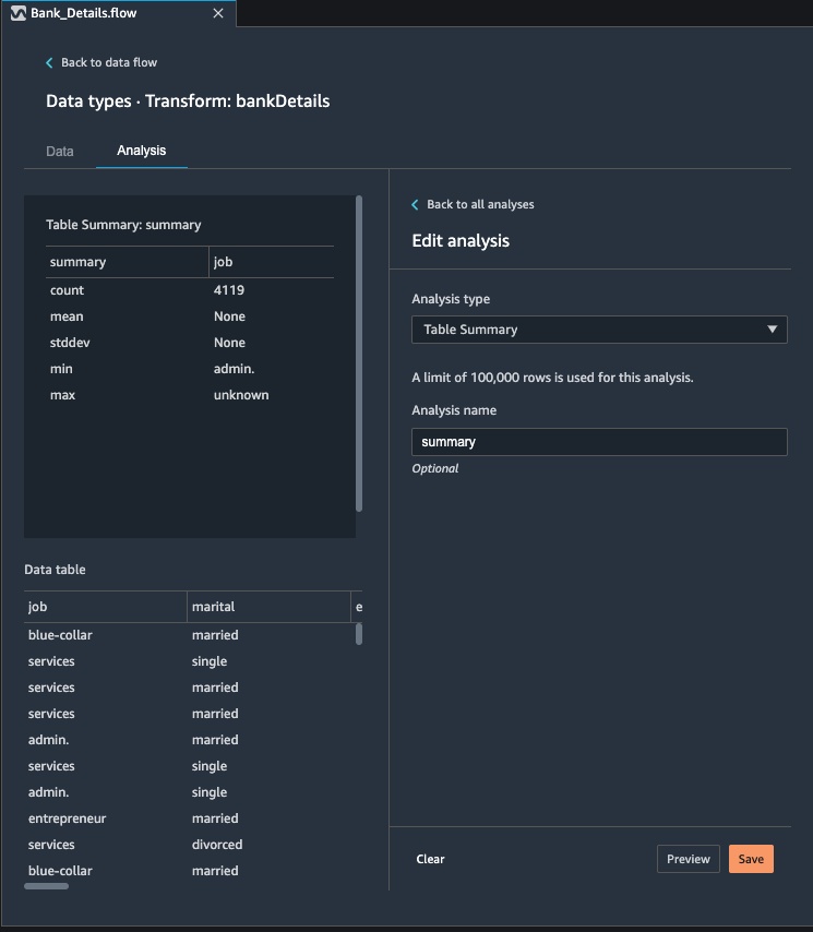
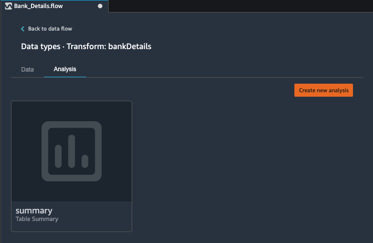
As part of data preparation for Machine learning, Kim starts analyzing the data. First she wants to generate the summary stats for Banking data set as she wants to understand demographics about her data set, for example, what is the average age of the clients. |
Under Data flow tab
|
|
|
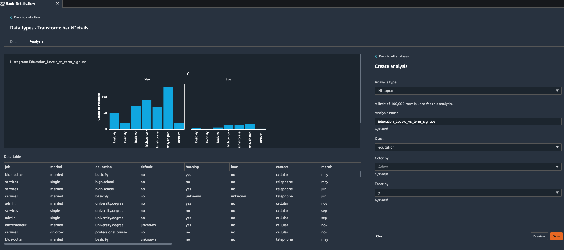
After looking at summary stats, Kim now wants to create a histogram to understand how different education levels of her clients is distributed against longer term deposit sign ups. For this Kim decides to use built in histogram feature of Data Wrangler tool.
Kim uses histogram chart to visually inspect if education levels and longer term opt-ins have any uneven distribution. |
Under Data flow tab.
|
Kim observes clients who have University Degree have most opt ins and clients who have basic education have low number of opt ins. |
| Next, Kim wants to know if there are any missing values in her banking data set, for this she decides to use custom transformation feature available in Data wrangler tool and apply pandas df.info() method on Banking data set. |
Under Data flow tab
|
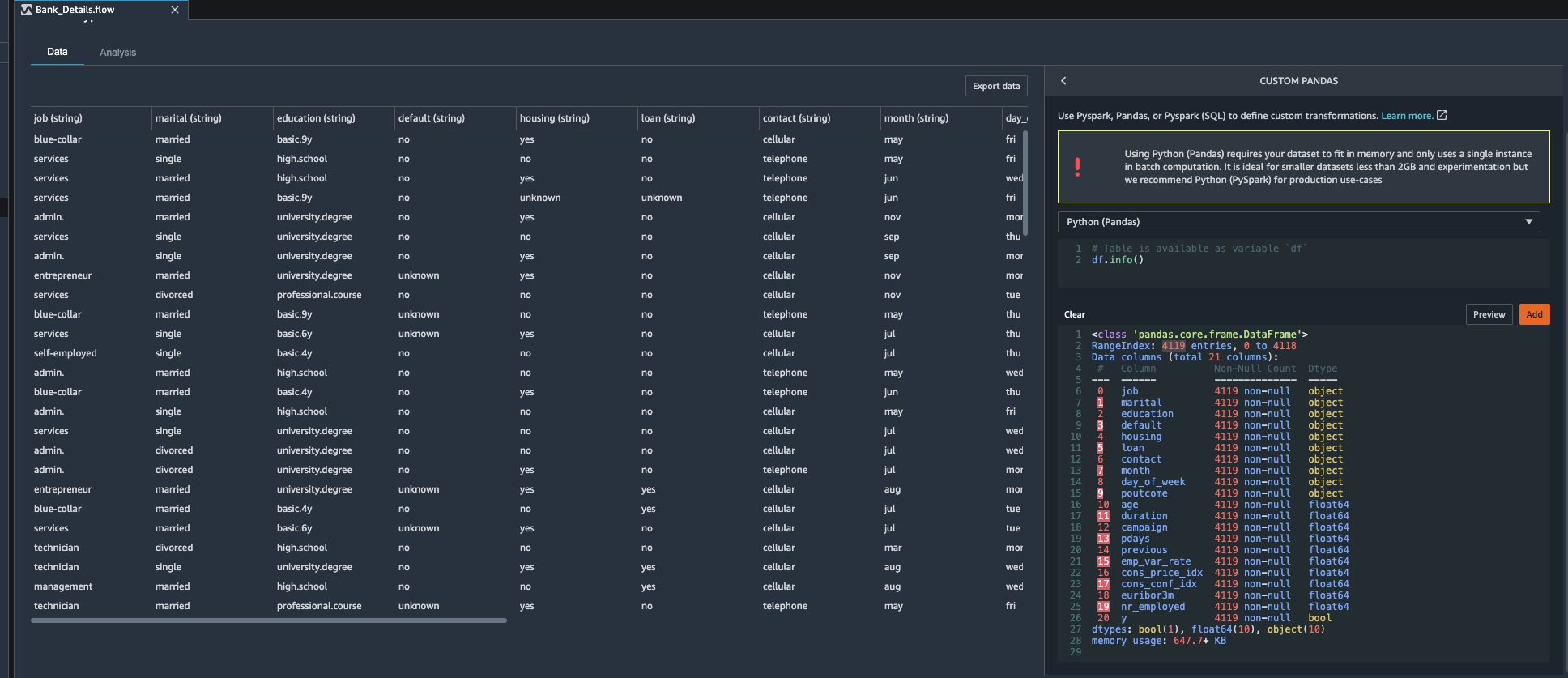
Kim observes that total number rows in this data set are 4,119. She also notices that each column has same number of values present. Kim decides that she does not need to drop any columns. |
Drop Unused Columns
| Say | Do | Show |
|---|---|---|
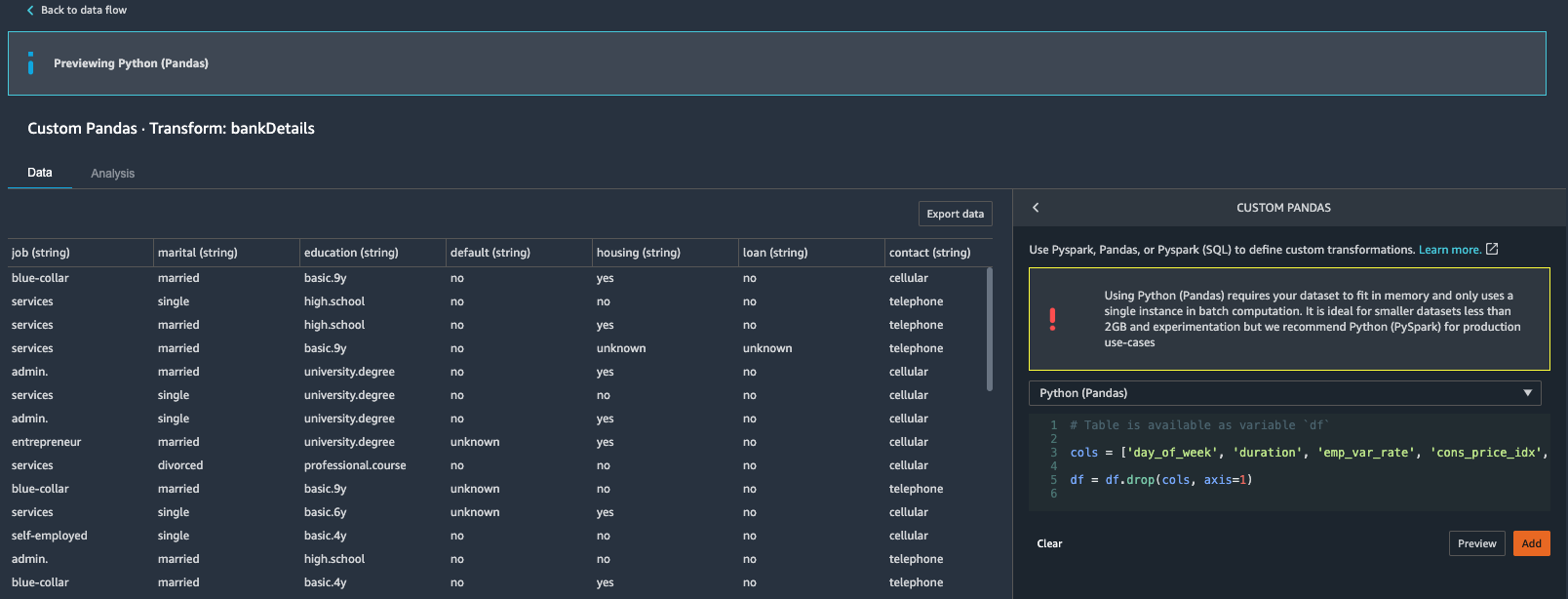
| As kim goes through the banking data set, she observes that some fields especially socio-economic data can be dropped from the data set in her first iteration of data modelling, so she decides to drop social economic fields and other campaign related fields. Fields that Kim wants to drop are: day_of_week, duration, emp.var.rate, cons.price.idx, euribor3m, nr.employed |
Under Data flow tab.
A new transformation step is now added to the flow.
|
|
Create Dummy Variables
| Say | Do | Show |
|---|---|---|
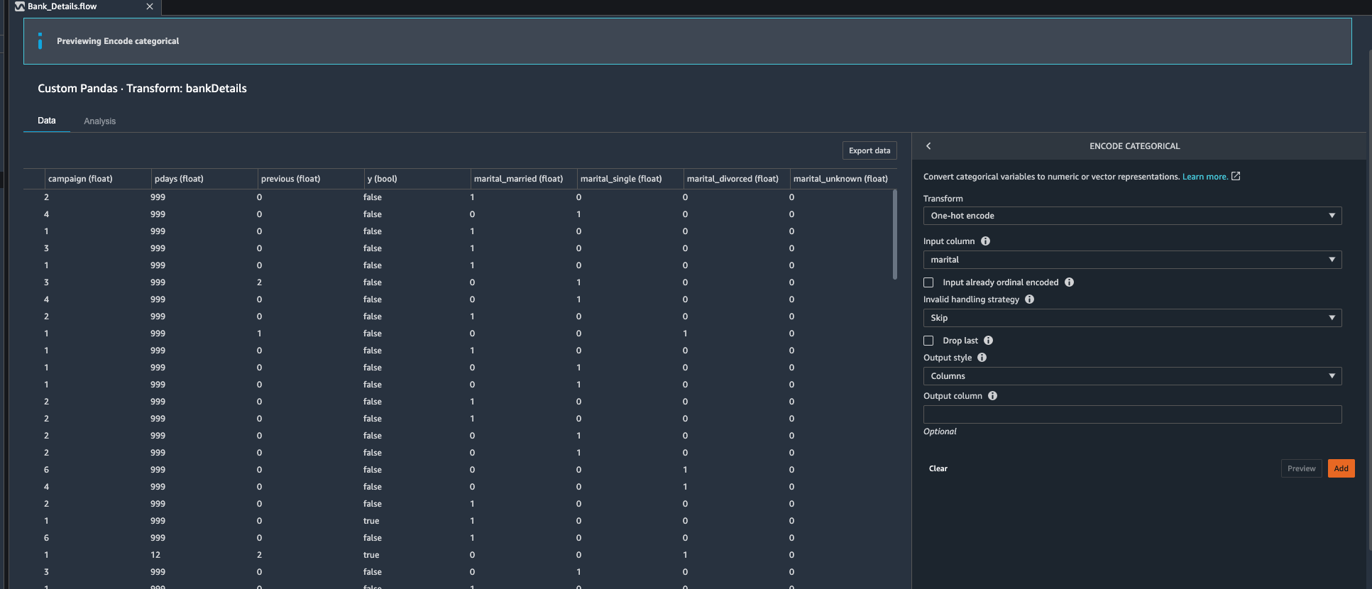
| Kim observes there are many dummy variables in banking data set, she decides to use Data wrangler to use built in encoding feature to create reference variables. Kim identifies following categorical feature that she want to create dummy variables for following Categorical Variables: job, marital , education, default, housing , loan , contact, month. | git stu
Under Data Flow.
|
|
Standardizing Numeric Variables
| Say | Do | Show |
|---|---|---|
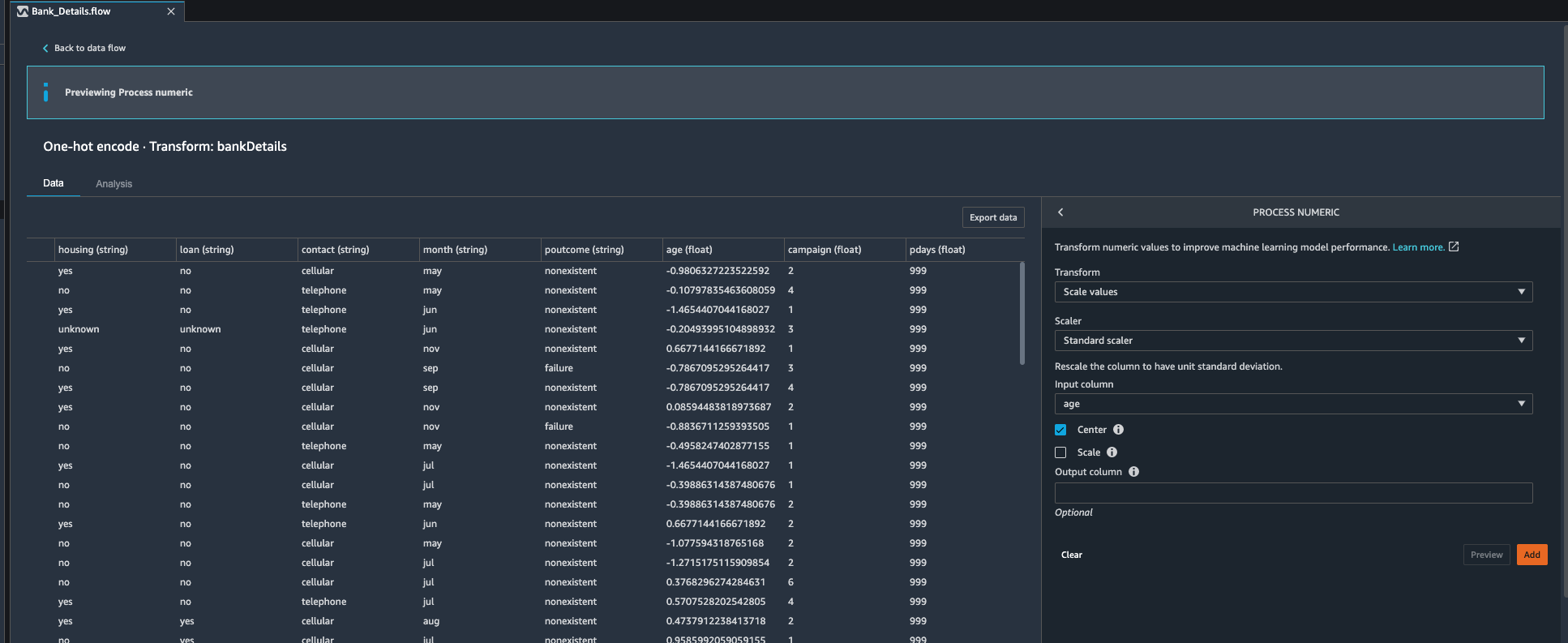
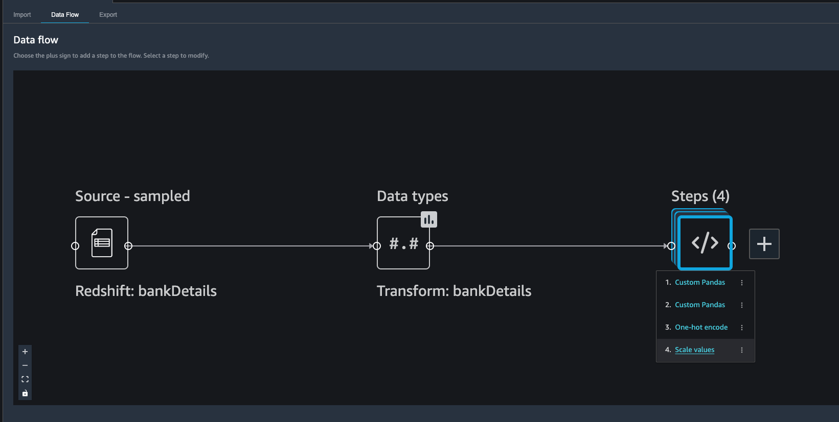
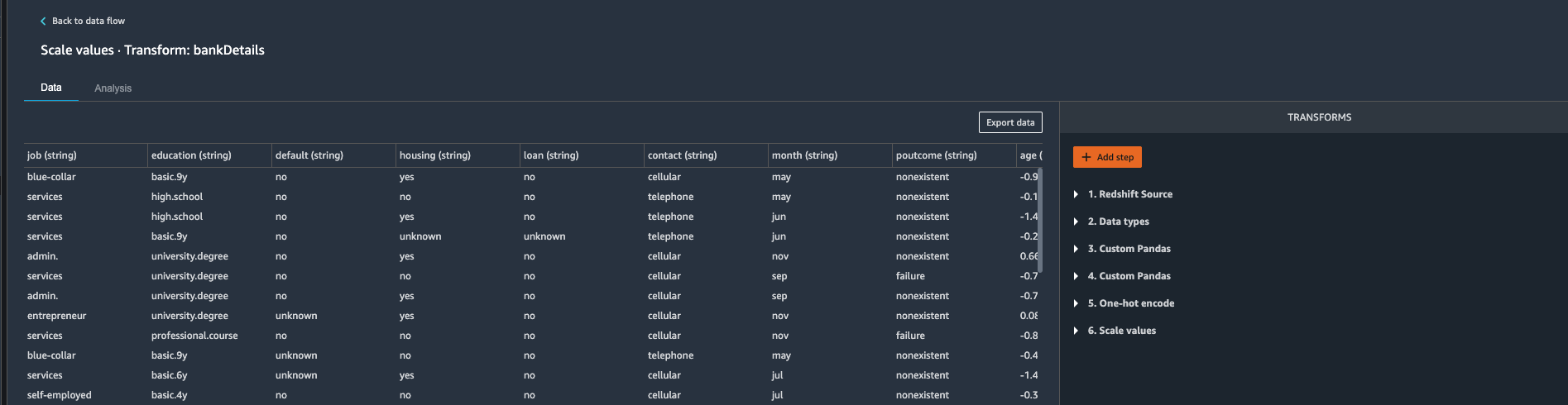
| Kim now decides to tackle numeric features. Since Kim is planning to use Gradient descent algorithm she knows that she need to work on feature scaling. She observes that age, campaign, previous, pdays columns are of numeric type that need to go through standardization process. She decides to use Data Wrangler’s built in transformation “Process Numeric” to tackle this challenge. |
Under Data Flow.
|
If notice the |
Export Processed Data
| Say | Do | Show |
|---|---|---|
| Kim has completed her challenge now, she has finished analysis, feature encoding and feature scaling. Now she decides load this Data back to data warehouse where she can use Redshift Machine learning to train a classification model. |
Under Data Flow.
|
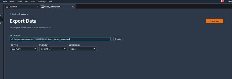
|
Next Steps
| Say | Do | Show |
|---|---|---|
|
Kim now has machine learning ready data on s3.
Kim can utilize Redshift ML or Amazon Sagemaker Studio to train a machine learning model. |
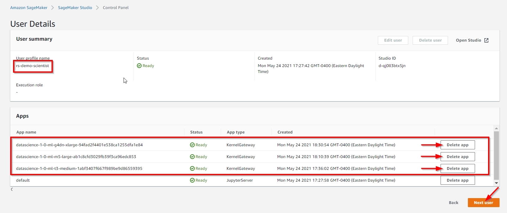
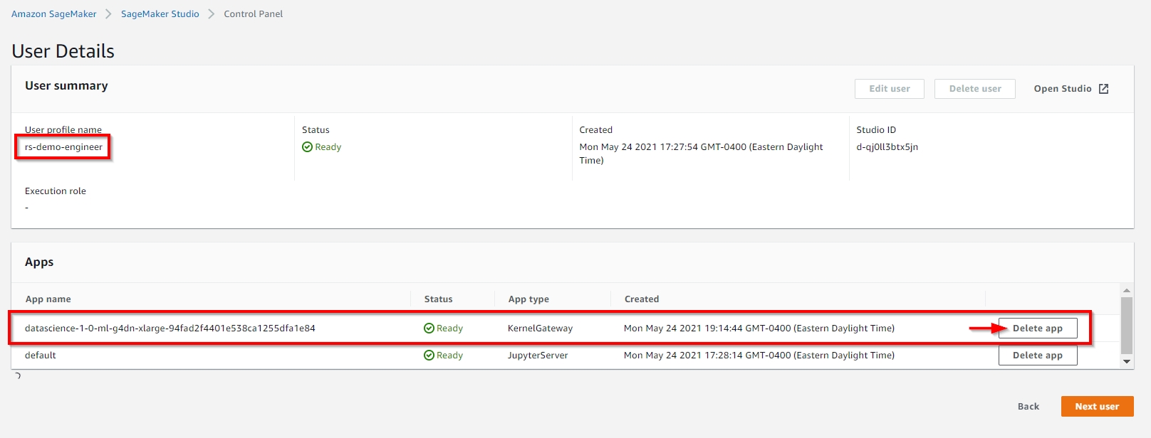
Before you Leave
Since only one domain is allowed per account per region, you cannot launch multiple Studio demo stacks in same account, region.
| Step | Visual |
|---|---|
You need to manually delete all the non-default apps under both rs-demo-scientist and rs-demo-engineer user profiles, before you can delete this stack, as shown below. |
   |
If you are done using your cluster, please think about deleting the CFN stack or to avoid having to pay for unused resources do these tasks:
- pause your Redshift Cluster
- stop the Oracle database
- stop the DMS task